고정 헤더 영역
상세 컨텐츠
본문

본 게시글은 강필성 교수님의 다변량 데이터 분석 강의를 기반으로 작성되었습니다.
작성자 : 16기 최규빈
6) Artificial Neural Networks
Perceptron
Brain Structure
인간의 뇌는 뉴런 사이의 전기신호를 통해 메시지를 전달
- 여러 뉴런으로부터 신호를 받아 다른 뉴런으로 보내는 형식
사람의 뇌를 모사해서 컴퓨터에 표현하자!
Perceptron
An organism with only 1 neuron

$x_0$ = 상수
$x_1, x_2$ = 변수
$w_0, w_1, w_2$ = 가중치(학습 대상)
$h$ = 활성화함수
$y$ = 추정치
$t$ = 실제값(target)
$L$ = loss function
진행 과정
전반부
가중치와 변수를 곱한 후 더해 스칼라 값으로 만들어 줌
후반부
해당 값을 활성화 함수에 통과시켜 변환 후 넘겨줌
- Perceptron의 핵심
- 비선형(non-linear)을 거쳐야만 함
Perceptron의 관점
Input node
Input variables
- $x_0, x_1, x_2$ 각각을 Input node, 전체를 layer로 표현
Hidden node
Take the weighted sum of input values and perform a non-linear activation
- 여러 변수들의 정보를 가중합으로 더한 후 다음 단계로 전달할 양을 정함
Role of activation
previous layer의 정보들이 다음 단계로 넘길 때 전달할 양을 결정해준다
- non-linaer function을 사용하는 순간 다중선형회귀와 일치하게 됨
활성화 함수의 종류

- Sigmoid
Logistic / Logit 함수라고도 표현
- [0, 1]의 range, 학습속도가 느림
- 미분 시 0에 가깝게 나올 수 있음
- Tanh
- [-1, 1]의 range, 학습속도 상대적으로 빠름
- 미분 시 0에 가깝게 나올 수 있음
- ReLU(Rectified linear unit)
- max(0,a)
- 속도가 빠름 0으로 수렴X
Purpose of perceptron
input x와 target t 사이의 관계를 잘 설명하는 weight w를 찾는 과정
측정 방법
loss function을 통해 확인
Regression
주로 squared loss 사용
Classification
주로 cross-entropy 사용
- label을 더 높을 확률로 추정할수록 적은 loss
Cost function
loss는 개별적인 값, cost는 모델 전체적인 값에 대한 설명
Gradient Descent

Blue line : minimize 해야 하는 목적함수
Black circle : 현재의 solution
화살표의 방향 : 현재 solution의 qulity를 올리기 위해 움직일 방향
Gradient : 1차 미분값
- 현재 Gradient가 양수이므로 Cost를 낮추기 위해서는 x축 방향으로 왼쪽, 즉 w를 감소시켜야 함
방법론
1. 현재 gradient가 0인가?
Yes -> 학습 종료
No -> 학습 진행
2. gradient가 0이 되기 위해 어떻게 해야 하는가?
gradient와 반대 방향으로 current weight를 이동한다
3. 얼마나 움직여야 하는가?
Not sure
- 조금씩 이동하며 수렴을 기대한다
Theoretical Background
아주 작은 w의 변화율에 대해
$$
f(w + \Delta w) = f(w) + \frac{f'(w)}{1!}\Delta w + \frac{f''(w)}{2!}\Delta w + \cdots
$$
$$
w_{new} = w_{old} - \alpha f'(w),\quad where; 0 < \alpha < 1
$$
$$
f(w_{new}) = f(w_{old} - \alpha f'(w_{old})) \cong f(w_{old}) - \alpha|f'(w)]^2 < f(w_{old})
$$
Use chain rule
$$
\frac{\partial L}{\partial y} = y-t \quad \frac{\partial y}{\partial h} = 1
$$
$$
\frac{\partial h}{\partial a} = \frac{exp(-a)}{(1+exp(-a))^2} = \frac{1}{1 + exp(-a)} \cdot \frac{exp(-a)}{1 + exp(-a)} = h(1-h)
$$
$$
\frac{\partial a}{\partial w_i} = x_i
$$
Gradients for w and x
$$
\frac{\partial L}{\partial w_i} = \frac{\partial L}{\partial y} \cdot \frac{\partial y}{\partial h} \cdot \frac{\partial h}{\partial a} \cdot \frac{\partial a}{\partial w_i} = (y-t) \cdot 1 \cdot h(1-h) \cdot x_i
$$
$$
{w_i}^{new} = {w_i}^{old} - \alpha \times (y-t) \cdot 1 \cdot h(1-h) \cdot x_i
$$
- 현재의 출력값(y)과 정답(t)이 차이가 많이 날 수록 가중치를 많이 업데이트
- 대상 가중치와 연결된 입력 변수의 값이 클 수록 가중치를 많이 업데이트
Issue 1
얼마나 자주 가중치를 업데이트 하는가?
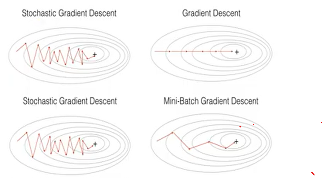
Stochastic Gradient Descent(SGD)
개별적 instance를 가지고 weight update
Batch Gradient Descent(BGD)
모든 instance를 사용해 loss를 평균낸 후 한번에 weight update
Mini-Batch Gradient Descent
SGD와 BGD의 절충안
N개의 instance를 사용해 weight-update
Issue 2
한번에 얼마나 업데이트 하는가?
$\alpha$가 너무 클 경우, 발산 가능성 있음
$\alpha$가 너무 작을 경우, 너무 느림
적절한 learning rate 필요
Adam, RMSProp 등의 방법론 자주 이용
Multi-layer Perceptron(MLP)
Limitation of Linear Model
1. Classification
Linear한 Hyper plane으로 구별
- Linear class boundary만 생성 가능
2. Regression
Multiple linaer regression
- 변수간 linear relationship 설명가능
비선형 관계의 예측이 불가능하다
Combine multiple perceptrons!
복잡한 문제를 작고 간단한 문제들오 decompose하자
Decision boundary of MLP
| Logistic Regression | Decision Tree | MLP | |
|---|---|---|---|
| No. of lines | 1 | No restriction | User defined |
| Direction of lines | No restriction | Vertical to an axis | No restriction |
Basic Structure
Feed-forward Neural Network with One Hidden Layer
Regression

The output node is a combination of all perceptrons
Classification

N. of output nodes = N. of classes
The role of hidden nodes
인공 신경망(ANN)의 복잡도(complexity) 결정하는 역할
Goal
best prediction을 만들어내는 weight를 찾는 과정
Features
- 순전파-역전파 과정을 모든 record를 반복하며 작동
- 매 step마다 actual target과 prediction을 비교
- 비교된 차이는 output node의 error
- error는 모든 hidden node로 전달되어 가중치를 업데이트함
Why it works
- 큰 error는 큰 weight의 변화를 이끌어냄
- 작은 error는 상대적으로 작은 변화를 이끌어냄
- error가 무시할만큼 작아졌을 때 weight 변화 중단
Common criteria to stop updating
- 가중치 변화율이 충분히 작을 때
- 지정한 Threshold 보다 misclassification rate가 적어질 때
- 지정한 epoch 수에 도달했을 때
Overfitting
너무 많은 iteration은 overfitting을 유발
How to avoid
- validation data를 tracking한다
- iteration을 제한한다
- network의 complexity를 줄인다
- N. of hidden layers, node를 조절한다
'심화 스터디 > 다변량 분석 스터디' 카테고리의 다른 글
| Chapter 8. Association Rule Mining (1) | 2023.05.11 |
|---|---|
| Chapter 7. Ensemble Learning (1) | 2023.05.11 |
| [다변량 데이터 분석] Chapter.05 (0) | 2023.03.28 |
| [다변량 데이터 분석] Chapter.04 (1) | 2023.03.21 |
| [다변량 데이터 분석] Chapter.03 (0) | 2023.03.19 |


댓글 영역